Tissue class segmentation
A very, very brief introduction to Bayesian probability
I will add more to this section at some point. But there are a few practical things about Bayesian statistics that are helpful in thinking about tissue class segmentation:
- At the end of the day you get a probability of a result being true (the posterior).
- This probability is based on both your prior knowledge (the prior) and the data at hand (the likelihood).
- Both prior knowledge and current data are expressed as distributions (i.e., neither are perfect, and thus both have some variance or error associated with them).
See, e.g., http://www.scholarpedia.org/article/Bayesian_statistics, especially Figure 1 on that page.
This is relevant because SPM (and other software) generally take a Bayesian approach to tissue class segmentation, and it’s helpful to have at least a general idea as to what this means.
Voxel intensities vary across tissue types
Consider a T1-weighted structural image. The information that is available from this image to separate tissue classes is the voxel intensity: different tissue types give off different strength signals, leading to different intensities. In a T1-weighted structural image, white matter is the brightest, followed by gray matter and CSF.
At first glance it might appear trivial to decide whether a portion of an image belongs to, say, white matter (WM) or gray matter (GM). However, sometimes this is not obvious on a voxel-by-voxel level due to variations in voxel intensities. Some of these variations may be due to biological variability or measurement error, but a fair amount can be attributed to partial volume effects. Partial volume effects occur when a voxel spans more than one tissue (or signal) type, as illustrated below.
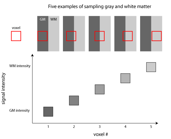
An illustration of partial volume effects. In this schematic figure, a portion of the brain containing both gray matter (GM) and white matter (WM) is sampled 5 different times using the same voxel. Because the resolution of our signal is determined by the voxel size, the final signal is an average of the different signals present within that area. The signal intensity of the voxel can thus reflect purely gray matter or white matter, or intermediate cases where it overlaps more than one tissue class. Note that the signal intensity is related to the volume of each tissue class contained in the voxel (e.g., the voxel that is 50% gray matter and 50% white matter by volume has an intensity that is halfway between the gray matter and white matter intensities).
It is particularly for these intermediate cases in which a probabilistic approach becomes very helpful. Intensities that are clearly gray matter or white matter can be assigned a high probability fairly easy; intermediate cases can be assigned probability values in the middle for multiple tissue classes, reflecting partial volume effects. Note that these intermediate values are thus proportional to the volume of a tissue class contained in a voxel.
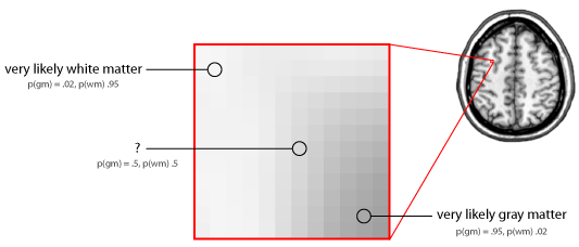
An enlarged section of approximately 12x12 voxels from a structural MRI image that spans a boundary between gray matter (GM) and white matter (WM). Extreme intensities are relatively easy to assign (though not with complete certainty), which results in high probability values. However, voxels whose intensity lies in the middle are more difficult, and the probabilities reflect this (in this case, equally divided between gray and white matter).
So, it’s important to note that the output from tissue class segmentation is not an absolute map of tissue class types; rather, for each voxel, it is a set of probabilities across all tissue classes to which that voxel may belong.
Distributions of voxel intensities
One way to think about voxel intensities is a distribution over the entire brain. However, with the knowledge that different tissue types give off different strength signals, this can be more accurately defined as a set of distributions—one for each tissue type. Thus, to model the distribution of voxel intensities, we just need to know something about the form of these underlying distributions.
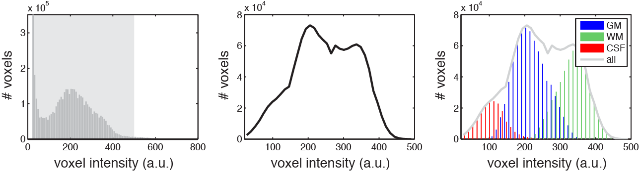
Voxel intensities in an example T1-weighted structural MRI image. Left: Distribution of all voxels in the image. Middle: Distribution of a subset. Right: Showing that the middle distribution (plotted again in light gray) is actually composed of three separate distributions: gray matter (GM), white matter (WM), and CSF voxels. Note that the number of tissue types in an actual structural image is greater, though the principles are the same.
One simple assumption would be that each tissue class conforms to a Gaussian distribution. This isn’t quite true, to typically (e.g. in SPM) they are modeled as combinations, or mixtures, of two ore more Gaussians. Describing a distribution as a combination of Gaussians is also referred to as Gaussian mixture modeling. So, with some idea about how many tissue classes are present, and the distribution of intensities likely to be in each tissue class, intensity information can be used to determine a likely tissue class for each voxel. However, if we can incorporate more information, we will come up with a better answer.
Bias and correcting for it
We have already seen that tissue class affects signal intensity, and that this relationship is one of the things we can use to segment a structural image. However, tissue class is not the only thing that can affect signal intensity. Another source of variability in signal intensity comes from bias (or “intensity nonuniformities”) in MRI images. This effectively means that some parts of the brain (regardless of tissue type) are likely to be brighter than other parts. Bias fields tend to vary smoothly (i.e., at a low spatial frequency), which helps in their estimation and removal. It is important to correct for intensity nonuniformity prior to (or as part of) segmentation so that it does not influence the assignment of tissue class probability.
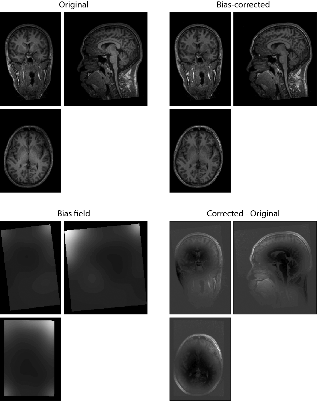
The original and bias-corrected versions of a T1-weighted structural image are shown in the top row. Note that even small differences (i.e. not apparent in visual inspection) can significantly affect the segmentation algorithm. At bottom left is the estimated bias field, and at bottom right the subtraction of the original image from the bias-corrected image, showing widespread differences.
Tissue probability maps
The intensity of voxels in an image is one type of information we can use in tissue class segmentation. Another type of information we have available comes from the fact that there are many features that most brains have in common regarding the spatial distribution of tissue classes. That is, tissue types aren’t randomly distributed in the brain, but they follow a relatively systematic organization, and we can use this information to improve our segmentation. Tissue probability maps are probability maps for different tissue classes constructed from a large number of brains that are registered into a common space. In a Bayesian framework, these maps represent the prior probability of any voxel belonging to a particular tissue class, and thus these are often referred to as “priors”.
Many tissue class segmentation algorithms make use of 3 tissue probability maps: gray matter, white matter, and CSF (and an implicit “other” category). Voxels that belong to other tissue classes (such as skull or soft tissue) can get incorrectly assigned to gray matter, white matter, or CSF, reducing the accuracy of the segmentation.
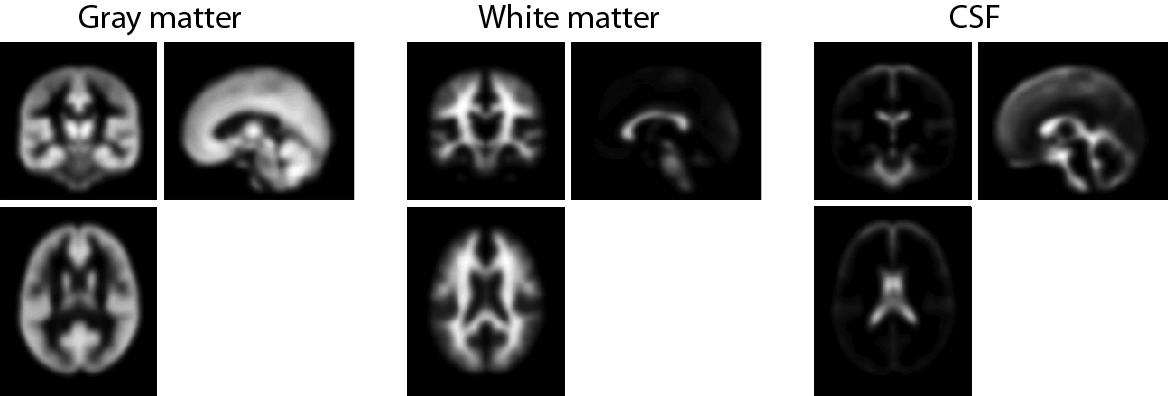
Tissue probability maps for gray matter, white matter, and CSF, as provided by ICBM. These reflect the probability of a voxel belonging to each tissue class based on the segmentation of a large number of young adult brains which have been normalized to standard space. These can be found in SPMDIR/apriori/.
The “new segment” option in SPM8 makes use of a greater number of tissue classes, adding skull and soft tissue.
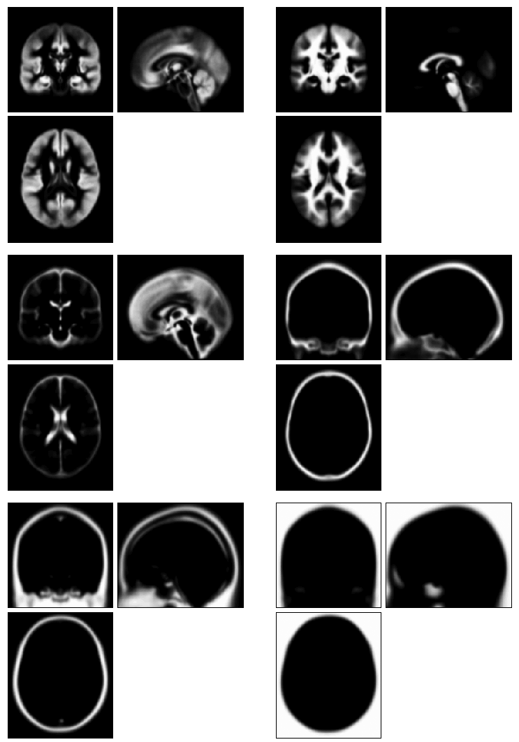
Tissue probability maps used by the “new segment” tool in SPM8. In addition to gray matter, white matter, and CSF, these include skull, soft tissue, and an explicit “other” category. These can be found in SPMDIR/toolbox/Seg/TPM.nii, which is a multivolume Nifti file (one volume for each of the 6 tissue classes).
“Unified segmentation”
A problem arises when using tissue probability maps to segment a subject’s image. That is that the tissue probability maps are in a standard space (in SPM, this is MNI space); however, the subject’s T1 image is not. Therefore, the registration between subject-space and MNI space must be computed before the tissue probability maps can be used. However, we might also want to use the tissue class segmentations to inform the segmentation (e.g., align gray matter in the subject’s image to gray matter in the template).
One approach for dealing with this is to incorporate spatial normalization and tissue class segmentation within the same model so that an optimal solution is found for both within the same framework. This “unified segmentation” approach, introduced by [AshburnerFriston2005], is what is used in SPM.
Optimizing starting estimates for normalization
After importing images into Nifti format, their orientation can be fairly far removed from standard space. In some cases this can prevent the segmentation routines from finding a good solution. Thus, it’s often helpful (and sometimes necessary) to reorient structural images so they approximately match standard space (though the “new segment” routine is probably slightly more robust to starting discrepancies). Reorientation can be done using the “display” tool and is covered in Using Display to reorient an image.
Tissue class segmentation in SPM
To segment an image using the old segmentation routine, press the “segment” button.
To segment an image using the “new segment” routine:
- From the batch editor go to the menu option SPM > Tools > New Segment.
- Under “Volumes”, specify one structural image (probably T1) for each participant.
- Each tissue class requires a tissue probability map (automatically filled in), the number of Gaussians used to model the distribution of voxel intensities for this tissue class type, and the types of output images requested. Most of the time writing out a native space gray matter image, and a modulated normalized gray matter image, will be sufficient. (Note: modulation is a separate topic that will be covered separately.) If you are planning on using DARTEL for image registration, select “Native + DARTEL imported”; The “DARTEL imported” generates rc* files that can be used with DARTEL.
- When this is set, press the green “run” button.
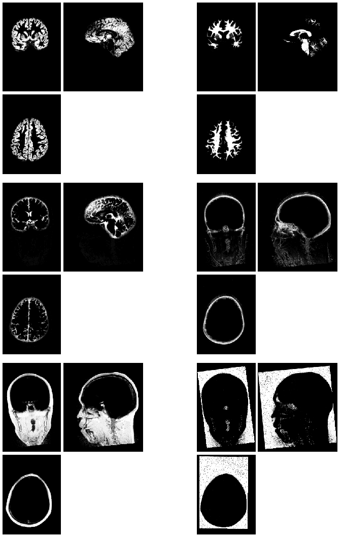
After segmentation, native-space images are produced that reflect each voxel’s probability of belonging to each one of the six tissue classes.
What to do when tissue class segmentation fails in SPM
When segmentation fails in SPM, it is often due to either particularly bad bias, or grossly inaccurate starting estimates for spatial localization. If segmentation fails, the following will usually fix it:
- Re-orient the structural image so that it generally matches the MNI template (see Using Display to reorient an image). N.B. If this is a functional MRI study, make sure to apply the reorientations to both the structural image and the functional images (you may want to use checkReg to ensure everything is properly aligned to make sure).
- Implement a two-pass bias-correction procedure. First, run segmentation without writing out any segmented images, but writing the bias-corrected image, which will be prepended with an “m”. Then, run segmentation again on the m* image, also writing out the segmented files to ensure that it worked properly.
Although it may be that only some subjects fail segmentation, it’s probably a good idea to follow the same protocol for all subjects to ensure that no bias is introduced through using different protocols.
