Multiple comparisons and how to deal with them

Why performing multiple comparisons present a challenge

Understanding the issues involved in multiple comparisons is really just a matter of thinking through the implications of standard statistical tests. For example, let’s say we have two groups of adults, basketball players and horse jockeys. We want to know if they differ in height. We do a t-test to compare heights, and the result is that the heights differ at a level of p < .05. We conclude that the heights in these two groups are likely to differ.

But what are we really looking at? We have two distributions of height, which we have sampled for each group. What we are interested in is whether the means of the population distributions differ. The p < .05 level suggests that with the data we have observed, 5% of the time the population means will not differ. Thus, 95% of the time with the observed data the populations are different, and we can be fairly confident in our interpretation.

Now let’s say that we do this test on 20 basketball players and horse jockeys, all from different countries. In every case we get a significant difference, p < .05. Are we justified in thinking that in every country there is a true height difference between the true groups?

Statistically, not really. Each time we perform this test, there is a 5% chance that we will find a difference when there really isn’t one. If we do the test 20 times, then, probability tells us that one of these tests is likely to be a false positive. The problem is that we don’t know which one!

In neuroimaging, the problem is exaggerated because we have so many more comparisons. Let’s say we have 10,000 voxels in our image and use a cutoff of p < .05 (uncorrected), and find to our delight that we have 500 significant voxels. It’s true that 500 significant voxels seems like a lot, until you realize that this is exactly the number we would expect by chance, even if there was no significant difference in the data. Because we are interested in discovering something about how the brain actually works, and not in interpreting random noise, we need to find a way to focus in on true differences in our data. This is what “correcting for multiple comparisons” is all about.

This issue was illustrated nicely by [Bennett2011]. The authors placed a dead salmon in the MRI scanner and requested that the fish complete a mentalizing task. The salmon was shown photographs of humans in situations that were designed to be socially inclusive or socially exclusive, and the salmon was asked to determine which emotion the human in the photograph was feeling. The data were processed using a standard analysis pipeline in SPM. Remarkably, at a voxelwise threshold of p < .001, the salmon showed significantly more brain activity during photo presentation than at rest (see below). The fact that these results seem intuitively implausible (!) underscores the reality of noisy data and false positive results. Gratifyingly, when Bennett et al. used a correction for multiple comparisons, there was no significant change in brain activation in the dead salmon.

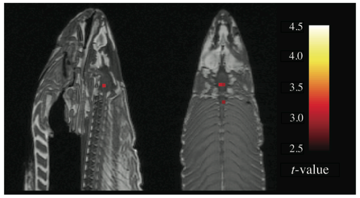
Figure 1 from Bennett et al. (2011) showing “activations” in the brain of a dead salmon who was presented with an experimental paradigm on perspective taking. These results are shown at p < .001 (uncorrected), but were not present when multiple comparisons were controlled for.

Principled control over false positives

The idea of “principled control” over false positive results is that the researcher (and the reader) have some idea about what the likelihood of a false positive result is. In the case of a single t-test, using a criteria of “p < .05” actually communicates this information—we know that the likelihood of a false positive result is 5%. If there are 10 such tests done, we would also know that the likelihood of a false positive has increased (over all tests) to 50%.

In brain imaging, the situation is often not as clear. As we have seen, the chance of a false positive result depends on both the threshold used, and the number of comparisons. But the number of comparisons is often not reported in neuroimaging studies. Thus, a threshold of p < .001 would result in a very different number of false positives in the case of 1,000 voxels vs. 10,000 voxels vs. 100,000 voxels. You might think of “principled control” as applying a threshold in a way that takes these differences into account.

Note that “principled control” does not necessarily mean “more stringent”. Rather, it simple indicates the level at which false positive results could be expected. For example, one could use an FWE-corrected voxelwise threshold of p < .20 threshold, which would indicate that the current results have a 20% chance of containing a false positive. This is much more informative than using an uncorrected threshold of p < .001, which does not give any information about the expected rate of false positives (though assuming the dataset contains at least 1,000 voxels, we know there is likely to be at least 1 false positive).

For an excellent overview of multiple comparison correction, see [Bennett2009].

Spatial correlation

One of the ways in which neuroimaging data differs from “standard” data is that data are spatially correlated. This means that in the case where you have 10,000 voxels, you are not performing 10,000 independent tests—rather, the number of independent tests is somewhat smaller, and will depend on the spatial correlation in your data.

“Spatial correlation” can also be though of as “smoothness”—smoother data shows more spatial correlation. This depends in part on the smoothing applied during preprocessing, but is also an intrinsic property of the MRI signal (and indeed the brain). The smoothness will be different for every dataset, and thus the appropriate statistical threshold will also differ. This is one reason why “rule of thumb” thresholds (e.g. “p < .005 (uncorrected) with a 10 voxel extent”) can be problematic: they may be appropriate for some datasets, but not others.

Ways of dealing with multiple comparisons

If you want

Bonferroni correction

One standard approach to correct for multiple comparisons is simply to divide the target false positive rate (typically .05) by the number of comparisons. Thus, if I’m conducting 5 tests, I would require each test to be significant at .05/5, or p < .01. Across the 5 tests my overall rate of expected false positive results would then be .05.

For neuroimaging, one approach would be to divide the target p value by the number of voxels. However, this tends to be overly conservative because there are typically far fewer independent tests than voxels (due to the spatial correlation of the data). Thus, Bonferroni correction per se is typically not used in whole-brain analyses. (However, it is still a viable option to control across a smaller number of ROIs, for example.)

Random field theory

In the early days of imaging it was discovered that brain images could be analyzed using random field theory (RFT). The idea is that if you assume an image consists of random Gaussian noise, you can determine whether the height of a peak (e.g. a voxel) is higher than expected, or whether the size of a cluster is bigger than expected. The peak-level correction in SPM, and the FWE cluster extent correction, rely on RFT.

One assumption of RFT is that the data in an image are, in fact, Gaussian. To meet this assumption, imaging data needs to be smoothed. A rule of thumb is that the smoothing should be at least 3 times bigger than the voxel size. So if fMRI data are acquired with 3mm^3 resolution, this would mean smoothing at ~9mm^3.

For a relatively intuitive introduction to RFT, see [Worsley1996].

False discovery rate (FDR)

FDR was introduced to the neuroimaging community by [Genovese2002]. The intuition behind FDR is that the proportion of false positive results is known. So, using a voxelwise FWE-corrected threshold of p < .05 means that the probability of any voxel being a false positive is 5% (hence, it is unlikely you are reporting any false positives). Using a voxelwise FDR-corrected threshold of q < .05 means that you expect 5% of your reported results to be false positives (hence, it is likely you are reporting false positives, but you know how many you are reporting).

Voxelwise FDR correction has become popular in many neuroimaging software packages. However, [Chumbley2009] point out that it does not control for false positive clusters, which are generally the features on which we make inferences. [Chumbley2009] make a compelling argument that a “topological FDR” is more appropriate; that is, using FDR to control the number of false positive clusters, rather than the number of false positive voxels. This approach is now the defaults in SPM8 and beyond.

Nonparametric (permutation) tests

Nonparametric approaches are processor-intensive, but make relatively few assumptions about the data, and are thus extremely powerful. The SnPM package will do these in SPM but is slightly unintuitive. In FSL, the randomise command does a very nice job.

[Nichols2001] has a nice review of nonparametric approaches.

Limiting the number of comparisons using anatomical hypotheses

The large number of voxels in the brain indeed means that effects often need to be fairly strong, or that a large number of subjects are needed, for them to reach whole-brain significance. However, for many hypotheses, whole-brain significance is not necessary. By incorporating a priori anatomical assumptions into our hypothesis testing, we can spatially restrict our statistical tests, reducing the number of comparisons for which we need to control.

As an extreme example, let’s say that I do a study that involves people listening to sentences. When I analyze the data, I contrast sentences > silence, and I find a large cluster of activation outside of the brain. In this case, it would be clear that I have an a priori belief that “activation will be in the brain”—thus, I just need to formalize this by only examining voxels in the brain. (Note that this is what SPM does by default, so hopefully this issue would not come up in real life!)

I may have a further expectation that the results I’m interested in will be in the temporal lobe. One way to incorporate this would be in a post-hoc way: perform a whole-brain analysis, and then lower the threshold until I see something in the temporal lobe. However, it is trivial to incorporate my “temporal lobe hypothesis” in a principled way by using an explicit anatomical mask for the temporal lobe. I can then correct for multiple comparisons within the region I am interested.

Put another way, your data don’t care that you are more interested in some brain regions than others—random noise and false positives are equally likely in areas you care about as elsewhere, even if you are more likely to consider them a “real” result when they appear to line up with your hypothesis. Exercising principled control over false positives helps protects you from being led astray.

For more ways to spatially restrict statistical comparisons, see Spatially restricting analyses.